In some scenarios you will need to create a many to many relationship in your cube in SSAS. One of the problems that arise from many to many bridge tables are the size of these tables. In this example we have a fact table that contains the history of a person and measures for that person at a bi weekly basis. Each person can be in a Program. Each person can be in more than one program at a time also. We have thousands of people so the fact table contains about 8 million rows.
Typically a bridge table will have a surrogate key for the dimension and a surrogate key to the fact table or a degenerate dimension based on the fact table. The key on the fact table in this case is the person id and the date key. So to create a many to many based on this key would be 8 million rows times the number of programs a person is in. There are over 300 programs, and some people are in as many as 6 programs at one time. This would make the bridge table over 24 million rows. This would also hurt performance quite a bit. I will admit that in some situation this type of bridge table cannot be avoided, but not here.
To create a bridge table that is much smaller all we need are all of the program combination that occur in our source data and come up with a unique key for each of those combinations.
The first step in this process is to look though the source data and determine all of the program combination. Each person has an program open date and close date. The fact table is at a bi weekly granularity, so we will check the programs at the same granularity.
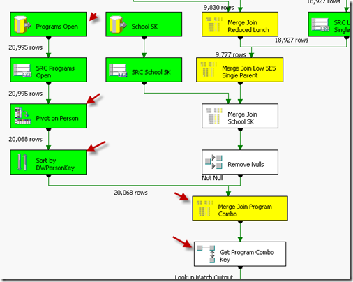
Here you see an SSIS package that will loop through each date in the past bi-weekly and determine which programs people were in at that time. This package is loading all history. If you are running your package on a nightly basis then you will only need to check the current date after this history is loaded.
Here is the data flow in this package.
The query to get the programs is below, The date is hard coded here but this would be either getdate() or a variable for the loop getting history.
With Programs as (
Select Distinct f.DimDWPersonKey, f.DimProgramKey
From FactSAMISPerson f
Where f.DimDWPersonKey > 0 and
f.EpisodeOpenDate <= ’2007-01-01′ and
isnull(f.EpisodeCloseDate,’9999-01-01′) > ’2007-01-01′)
Select ‘a’ + convert(varchar(3),ROW_NUMBER() Over(partition by DimDWPersonKey Order by p.DimProgramKey)) RowNum,
p.DimDWPersonKey, p.DimProgramKey
from Programs p
Order by p.DimDWPersonKey, p.DimProgramKey
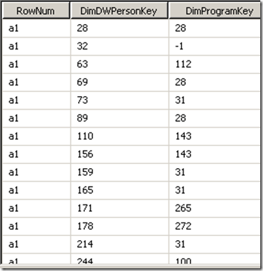
The pivot transform pivots on the person id. If you need to know how to use the pivot transform check out this article. So the incoming data looks like the following image:
The data after the pivot will look like the following image. Notice there is a person with two programs.
The reason for having 20 columns is to handle any situation where a person is in up to 20 programs at one time. This is way over kill because the highest in our data is 6 programs at a time. But you want to ensure that you can handle increases in the future.
The aggregate groups on all 20 program columns to eliminate duplicates. We do not need the person Id any more at this point so it is dropped. The lookup check the program combo table for duplicates. This ensures a unique id for each program combination and no repeats. Here is the program combo table.
Now every existing program combination is on this table and it has a unique id. The next step is to load the fact table and do a look up on this table to get the unique id. This is done using the same query above to load the program combo. Now you just need to do it for each person for each date you are loading in to the fact table. In the image below you can see this part of the fact table load. It works just like the package above, but this time is mapped to the incoming person id writing to the fact table. The lookup then gets the unique id by comparing all 20 columns in the query to all 20 columns on the program combo table.
The last step is to pivot the program combo table to create the bridge table. Here is the view used to do that.
SELECT ProgramComboID, ProgramSK
FROM (Select ProgramComboID, a1, a2, a3, a4, a5, a6, a7, a8, a9, a10, a11, a12, a13, a14, a15, a16, a17, a18, a19, a20 from ProgramCombos) as p
Unpivot (ProgramSK for id in (a1, a2, a3, a4, a5, a6, a7, a8, a9, a10, a11, a12, a13, a14, a15, a16, a17, a18, a19, a20 )) as s
Here are the results of that query.
Now you can add this view as the bridge table in your DSV for SSAS and create the relationships. This made the bridge table only 7404 rows. Much better than the 24 million we would have done with a traditional bridge table load.


