When building a SSAS cube, you typically have a star schema containing dimension tables and fact tables. For dimension tables, you generally model these as one table per object. Building the dimension in the ETL system involves joining the various normalized description and hierarchy tables that populate the dimension attributes and writing the results into a single table. Creating a single denormalized dimension table will result in a performance gain when processing a cube, as well as simplifying your star schema (avoiding having to use a snowflake schema).
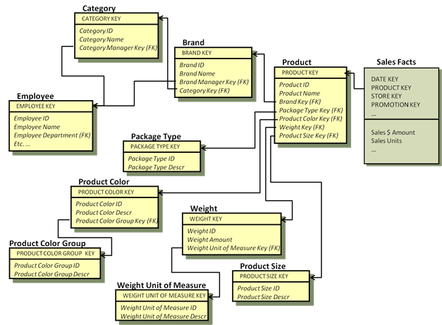
The figure below shows an example of typical product-related attributes in a normalized model.
The base table is called Product and it connects to the Sales fact table at the individual product key level. From this set of tables, it’s possible to create an analytic calculation such as SUM([Sales $ Amount]) by CategoryName, or by ProductColorGroupDescr, or any other attribute in any of the normalized tables that describe the product. It’s possible, but it is not easy.
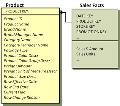
In the dimensional version of the Product table, we would join the product-related tables from the figure above once, during the ETL process, to produce a single Product dimension table. The below figure shows the resulting Product dimension based on the tables and attributes from the above figure.
To save development time at the cost of decreased performance, instead of creating a new denormalized table in ETL, simply create a view in SQL Server or a named query in SSAS that performs all the necessary joins.
From the single Product dimension table it is still possible to calculate SUM([Sales $ Amount]) by CategoryName, or by ProductColorGroupDescr, or any other attribute in the Product dimension, which includes all the product related attributes from the normalized model. Note that the two models are equivalent from an analytic perspective.
Usability is significantly improved for BI application developers and ad-hoc users with the denormalized dimensional table. In this simple example, the ten tables that contain the 12 product attributes are combined into a single table. This 10 to 1 reduction in the number of tables the user (and optimizer) must deal with makes a big difference in usability and performance. When you apply this across the 15 or 20 dimensions you might typically find associated with a Sales business process, the benefits are enormous.
The main difference between the two approaches is that the normalized version is easier to build if the source system is already normalized; but the denormalized dimensional version is easier to use and will generally perform better for analytic queries.
Using BI Tools to Mask Complexity
Some BI tools have a metadata layer that can be used to display a normalized physical model as if it were a denormalized dimensional model. This does meet the usability requirement, but it usually has a price. First, it only works for those users working with the specific tool. Any other access, such as queries embedded in applications, will need to work with the normalized model. Second, this metadata layer puts these tools in the role of creating complex SQL, which is often poorly formed. In which case, the user is usually reduced to writing the SQL by hand. Third, the underlying physical model is still normalized, which may not perform well for analytic queries compared to the denormalized dimensional model. A fourth cost is in actual dollars; these tools are fairly expensive.
More info:
Implementing a Microsoft SQL Server Parallel Data Warehouse Using the Kimball Approach


