

Introduction
All big data systems are not made equal, including SQL-on-Hadoop systems like Hive, Polybase and SparkSQL. All of these employ various distributed computing techniques. In this article we learned why it is critical to understand some of these techniques in other to make the right big data tool selections.
In Part I of this series we learnt what gave rise to Hadoop and the need for SQL-on-Hadoop big data systems which was pioneered by Hive. We also looked at the internal relational database in the Hive architecture and how it interacts with Hadoop. We further looked at some Hive database objects, data types and how to load data into Hive.
In Part II we will look at HiveQL Queries and other advanced features where anyone with T-SQL knowledge can perfect. We will look at some of the more common HiveQL- ANSI standards like CASE statement and JOINs. We will also explore some more advanced features like Bucketing, Partitioning, Built-in function and Streaming. All files referenced in this content can be found in the attached zip folder.
Querying with HiveQL
To demonstrate some of the more common HiveQL- ANSI standards, below are some typical queries with ANSI SQL logical steps most folks on this forum should be familiar with.
Logical query steps with case-statements
hive >
SELECT COUNT(id) as Cnt,
Gender,
CASE WHEN YearlyIncome < 50000.0
         THEN 'low' WHEN YearlyIncome >= 50000.0 AND YearlyIncome < 75000.0 THEN 'middle'
       WHEN YearlyIncome >= 75000.0 AND YearlyIncome < 150000.0
           THEN 'high' ELSE 'very high'
       END AS salaryBracket
from gamblers
WHERE  YearlyIncome>20000
GROUP BY  Gender,
CASE WHEN YearlyIncome < 50000.0
         THEN 'low' WHEN YearlyIncome >= 50000.0 AND YearlyIncome < 75000.0 THEN 'middle'
       WHEN YearlyIncome >= 75000.0 AND YearlyIncome < 150000.0
        THEN 'high' ELSE 'very high'END ORDER BY Gender;
This returns:
OK
Cnt     gender  salarybracket
4       F       middle
2       F       low
2       M       middle
3       M       low
Time taken: 39.248 seconds, Fetched: 4 row(s)
Subqueries:
hive >
Select
x.cnt,
x.Gender,
x.avg
From (
select COUNT(id) as cnt
, Gender
, avg(YearlyIncome) AS avg
from gamblers
WHERE YearlyIncome>20000  and  Gender ='F' GROUP BY Gender
ORDER BY Gender
)x
WHERE x.avg < 150000;
Results:
OK
x.cnt   x.gender        x.avg
6       F       55000.0
Time taken: 43.391 seconds, Fetched: 1 row(s)
Joins
Hive implements standard familiar ANSI joins (like in T-SQL) with a few restrictions. For instance Hive only supports equi-joins, which means that only equality can be used in the join predicate. However you can join on multiple columns in the join predicate as shown in the examples below.
Inner Join
hive >Select g.*, w.*
from winnings w
Inner join gamblers g
On g.Id=w.Id
and w.Amount>50;
Outer Joins
hive > Select g.*, w.*
from gamblers g
Left Outer join winnings w
On g.Id=w.Id;
hive >
Select g.*, w.* from gamblers g
Right Outer join winnings w
On g.Id=w.Id;
Full outer join
hive > Select p.*, l.* from gamblers g
Full Outer join winnings w
On l.Id=p.Id;
Semi joins
Unlike T-SQL and other dialects, Hive currently doesn’t support the IN clause on subqueries. In its place Hive provide LEFT SEMI JOIN which does the same thing. For instance, in T-SQL, for the regular IN subquery we can determine Gamblers with wins as shown below.
Select * from Gamblers g
where g.Id IN (select distinct Id
               from winnings );
To achieve this in Hive the query above can be rewritten as follows:
hive >
SELECT *
FROM Gamblers g LEFT SEMI JOIN winnings On (winnings.id = g.id);
Note however that for LEFT SEMI JOIN queries, the right table (winnings) may appear only in the ON clause and it cannot be referenced in a SELECT expression, therefore Hive does not support correlated queries like the T-SQL.
Exporting Hive Data
We’ve established that Hive data are stored as files, therefore exporting Hive table data could just be copying a file or a directory to a different location using Hive or Hadoop as shown in the steps below.
From Hadoop: Copy the content of the dimgeographyusa table into the Temp folder on HDFS.
hadoop>hadoop fs -cp /hive/warehouse/sqlonhadoop.db/dimgeographyusa/*.csv /user/HDIUser/Temp
From Hive: Copy the content of the dimgeographyusa table into the Temp folder.
hive>dfs -cp /hive/warehouse/sqlonhadoop.db/dimgeographyusa/*.csv /user/HDIUser/Temp;
To export data directly from a query we can use INSERT and a specific DIRECTORY. In the example below one or more files will be written to C:\Temp\hmeOwn folder depending on the number of Reducers invoked when processing the MapReduce job(s) associated with the SELECT statement.
  INSERT OVERWRITE LOCAL DIRECTORY 'C:\Temp\hmeOwn'
  SELECT id, Name, wins
  FROM GamblerWins;
Hive writes data to the files serializing all the fields as string and using the same default encoding it uses for the table’s internal storage i.e. TEXTFILE, unless another option was specified in the table schema.
Note that, the OVERWRITE and LOCAL options have the same effect as we’ve seen in previous statements.
Optimization and Tuning
When running hive queries it is easy to forget that the queries are just abstraction. In other words, the statements are converted to and run as MapReduce jobs which can be very expensive on large datasets if not monitored. Because Hive queries will be running mostly on large dataset it is important to consider all hive optimization options available, a few of which we will look at below.
Join Optimization
The Hive optimizer tries to minimize the number of MapReduce jobs when performing join operations. However, most of the time, Hive will use a separate MapReduce job for each pair of columns in the join. One way Hive tries to optimize joins is by assuming that the last table in your query (from left to right) is the largest. By this basic assumption it will try to buffer the first tables and stream the last table joining on the individual records.
For instance in the query below if we know that the winning table is bigger than the gamblers table then the query should be re-written as below by switching the tables as below.
hive >
Select g.*, w.*
from winnings w
Inner join gamblers g
ON g.Id=w.Id
and w.Amount>50;
If the two tables are large data sets you should notice a substantial performance difference between the two queries. If you don’t want to worry about the order of tables in your queries all the time, Hive provides a STREAMTABLE hint you can use to explicitly notify the query optimizer on which table (normally the biggest table) that it should stream.
For instance, in the example below, the optimizer will stream the winnings table even though it is the first in the query.
  hive >
  Select /* + STREAMTABLE(w) + */ g.*, w.*
  from winnings w
  Inner join gamblers g
  ON g.Id=w.Id
  and w.Amount>50;
Map-side Joins
You can force the optimizer to attempt to cache all small tables in memory and stream only the large ones. By so doing, hive can look-up every possible match against the small tables in memory on the map-side, and therefore eliminate the reduce step implemented in most common join scenarios. This could be implemented explicitly in queries if you know the small table, and if you know it will fit into cache. The query below instructs the optimizer to fit the gamblers table into cache.
  hive >
  Select /* + MapJoin(g) */ g.*, w.*
  from winnings w
  Inner join gamblers g
  ON g.Id=w.Id
  and w.Amount>50;
In recent versions of the feature can be enabled by setting the property, hive.auto.convert.join, to true directly in your $HOME/.hiverc file. The default is false.
hive> set hive.auto.convert.join=true;
You can also configure the size of what Hive should consider as a small table (to fit into cache) in the context of this optimization feature. The default definition of the property (in bytes) is normally set to 25000000 as below.
hive> hive.mapjoin.smalltable.filesize=25000000
Note that Hive does not support the map-side optimization for right and full-outer joins.
.hiverc file
Some distributions might not come with the .hiverc file, in that case you can create it yourself and store it at these locations %HIVE_HOME%\bin or %HIVE_CONF_DIR% directory. Hive will search in that order.
The following are typical line items in a .hiverc file:
  set hive.cli.print.current.db=true;
  set hive.cli.print.header=true;
  set hive.exec.mode.local.auto=true;
  set hive.auto.convert.join=true;
  hive.mapjoin.smalltable.filesize=25000000
Hive automatically looks for this file in the HOME directory and runs the commands it contains. It is therefore convenient for commands that you run frequently.
EXPLAIN
As you become more familiar with Hive in the Hadoop ecosystem you might have to learn how Hive translates queries into MapReduce jobs to help you use Hive more effectively. A quick and easy way to generate query plan and other information is to use the EXPLAIN clause. It comes in handy during optimization. In the example below, the EXPLAIN clause prints the various job stages of the SELECT query.
  hive >
  EXPLAIN
  Select x.cnt, x.Gender, x.avg
  From (
          select COUNT(id) as cnt
            , Gender
            , avg(YearlyIncome) AS avg
         from gamblers
         WHERE YearlyIncome>20000  and  Gender ='F' GROUP BY Gender
         ORDER BY Gender
  )x
  WHERE x.avg <150000;
Results:
OK
STAGE DEPENDENCIES:
  Stage-1 is a root stage
  Stage-2 depends on stages: Stage-1
  Stage-0 is a root stage
STAGE PLANS:
  Stage: Stage-1
    Map Reduce
      Map Operator Tree
…
…
  Stage: Stage-0
Fetch Operator
limit: -1
Time taken: 0.06 seconds, Fetched: 81 row(s)
Optimization is a very comprehensive process that should include other processes like indexing not covered here. This process might also benefit from Partitioning and Bucketing which we cover next.
Partitioning
The general motives for partitioning data in Hive are similar to that in relational database systems. Partitions can help organize data in a logical manner or scale load horizontally besides other, all of which can make it faster to query or slice data.
In the following step, a new table, GeographyUSStsPart, is created and portioned on two columns using the PARTITIONED BY keywords:
  hive >
  DROP TABLE IF EXISTS GeographyUSStsPart;
  hive >
  CREATE TABLE GeographyUSStsPart(GeographyKey INT, City STRING, StateProvinceName STRING, EnglishCountryRegionName STRING, PostalCode STRING, SalesTerritoryKey INT, IpAddressLocator STRING)
  PARTITIONED BY (CountryRegionCode STRING, StateProvinceCode STRING)
  ROW FORMAT DELIMITED
  FIELDS TERMINATED BY ','
  LINES TERMINATED BY '\n';
In Hive, you manage partitions by loading the right dataset explicitly into the right partition. In the next steps, three partition are generated for each of the three states (NY, CA, IL) and csv files containing the dataset for each of the state is loaded from the local directory C:\temp\GeographyUS as shown below.
  hive >
  LOAD DATA LOCAL INPATH 'C:\temp\GeographyUS\DimGeographyUS_CA.csv'
  OVERWRITE  INTO TABLE GeographyUSStsPart
  PARTITION (CountryRegionCode ='US', StateProvinceCode='CA');
  hive >
  LOAD DATA LOCAL INPATH 'C:\temp\GeographyUS\DimGeographyUS_NY.csv'
  OVERWRITE INTO TABLE GeographyUSStsPart
  PARTITION (CountryRegionCode ='US', StateProvinceCode='NY');
  hive >
  LOAD DATA LOCAL INPATH 'C:\temp\GeographyUS\DimGeographyUS_IL.csv'
  OVERWRITE INTO TABLE GeographyUSStsPart
  PARTITION (CountryRegionCode ='US', StateProvinceCode='IL');
Remember that you are responsible to make sure the right data files with the right data subsets go into the correct partitions. Hive does not check to make sure if the dataset corresponds to the partition or not.
You can see all the partitions that exists on a table with the SHOW PARTITIONS command:
hive> SHOW PARTITIONS GeographyUSStsPart;
The results
Results:
OK
partition
countryregioncode=US/stateprovincecode=IL
countryregioncode=US/stateprovincecode=CA
countryregioncode=US/stateprovincecode=NY
Time taken: 0.076 seconds, Fetched: 3 row(s)
If you have a lot of partitions and you want to see if partitions have been defined for particular partition keys, you can further restrict the command with an optional PARTITION clause that specifies one or more of the partitions with specific values as in the example below:
  hive> SHOW PARTITIONS GeographyUSStsPart
  PARTITION(countryregioncode='US');
Results:
OK
partition
countryregioncode=US/stateprovincecode=IL
countryregioncode=US/stateprovincecode=CA
countryregioncode=US/stateprovincecode=NY
Time taken: 0.076 seconds, Fetched: 3 row(s)
You can also use the DESCRIBE EXTENDED Table statement to see the partition keys on a table. The partition information will appear under the Partition Information section of the table description results as shown in the example below.
hive> DESCRIBE EXTENDED GeographyUSStsPart;
Results: OK ....... # Partition Information # col_name data_type comment countryregioncode string stateprovincecode string .......
It is important to note that the partitioning process is also mostly file operation and management process in keeping with the schema-on-read system. For instance the partitions on the GeographyUSStsPart table created above should generate the directory and the file structure shown on Figure 1 below.
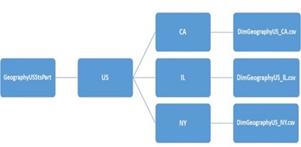
Figure 1: Folder and file structure of GeographyUSStsPart table partitioning.
If we list the subfolder under /hive/warehouse/sqlonhadoop.db/geographyusstspart/countryregioncode=US, we should currently see the three subfolders as shown in the example below. One subfolder for each of the three state partitions that we loaded data into with the LOAD DATA statement above.
hive>dfs –ls /hive/warehouse/sqlonhadoop.db/geographyusstspart/countryregioncode=US/;
Results:
Found 3 items
drwxr-xr-x  - fadje_000 hdfs   0 2015-10-11 21:49 /hive/warehouse/sqlonhadoop.db/geographyusstspart/countryregioncode=US/stateprovincecode=IL
drwxr-xr-x  - fadje_000 hdfs   0 2015-10-11 21:56 /hive/warehouse/sqlonhadoop.db/geographyusstspart/countryregioncode=US/stateprovincecode=CA
drwxr-xr-x  - fadje_000 hdfs   0 2015-10-11 21:48 /hive/warehouse/sqlonhadoop.db/geographyusstspart/countryregioncode=US/stateprovincecode=NY
Similarly, each of the state subfolders should also contain one of the three csv files that was loaded into each partitition. The example below lists the DimGeographyUS_NY.csv file that we loaded into the (CountryRegionCode ='US', StateProvinceCode='NY') partition above.
hive> dfs -ls /hive/warehouse/sqlonhadoop.db/geographyusstspart/countryregioncode=US/stateprovincecode=NY/;
Results:
Found 1 items
-rw-r--r--   1 fadje_000 hdfs       1105 2015-10-11 21:48 /hive/warehouse/sqlonhadoop.db/geographyusstspart/countryregioncode=US/stateprovincecode=NY/DimGeographyUS_NY.csv
Another thing to remember is that the partition keys (CountryRegionCode and StateProvinceCode) behave like regular columns, even though they are not part of the table definition. For example, the following query specifies the keys in the SELECT statement and returns them in the resultset, even though those two fields are not in the data files loaded into each partition.
hive>
SELECT CountryRegionCode, StateProvinceCode, City FROM GeographyUSStsPart
WHERE CountryRegionCode  = 'US' AND StateProvinceCode  = 'CA' LIMIT 5;
Results:
OK
countryregioncode       stateprovincecode       city
US      CA      Alhambra
US      CA      Alpine
US      CA      Auburn
US      CA      Baldwin Park
US      CA      Barstow
Time taken: 11.191 seconds, Fetched: 5 row(s)
Normally one of the most important reasons to partition data is for faster queries. In the query above, Hive scans the contents of one directory because of the WHERE clause. Therefore for very large data sets, partitioning can dramatically improve query performance. Partition keys implemented must represent common range filtering (e.g., timestamp ranges, locations etc.), i.e. they must be fields on which filtering (WHERE clauses) would be applied.
Warning: Queries that run across all partitions could result in huge MapReduce job if the table data and number of partitions are large. A very important safety measure against this is to put Hive in a Mode. In this mode, Hive will not allow queries against partitioned tables without a WHERE clause that filters on partitions to run. As shown below, by turning on this feature, the subsequent query fails, because the query did not have filtering based on the partitioned keys.
hive> set hive.mapred.mode=strict;
hive>
SELECT CountryRegionCode, StateProvinceCode, City FROM GeographyUSStsPart LIMIT 5;

Results:
FAILED: SemanticException [Error 10041]: No partition predicate found for Alias "geographyusstspart" Table "geographyusstspart"
However, If we reset the feature back to "nonstrict" mode as shown below, Hive gives the same query permission to run without the WHERE clause, .
hive> set hive.mapred.mode=nonstrict;
Bucketing
In certain situations, partitions may not offer the best way to separate out data and to optimize your queries. Bucketing is another option for decomposing data sets into more convenient parts to enhance query performance and data sampling. Note that bucketing can be applied to partitioned tables.
Bucketing tables enables more efficient queries because they exposes extra data segregation which the optimizer is able to employ. For instance, when two tables that are bucketed on the same columns include the columns in a join, the optimizer can efficiently implemented a map-side join.
Secondly, bucketed table make sampling more efficient. On Hadoop/Hive it is likely you will be working with large datasets, bucketing provides extra convenience for sampling and trying out your queries on a fraction of your dataset in exploratory data analysis.
To bucket a table we use the CLUSTERED BY clause to specify the columns to bucket on and then indicate number of buckets to be generated as shown below.
DROP TABLE IF EXISTS gamblersBkt;
CREATE TABLE gamblersbkt (
Id INT,
First STRING COMMENT ' First name',
Last STRING COMMENT  ' Last name',
Gender STRING,
YearlyIncome FLOAT,
City STRING,
State STRING,
Zip STRING)
CLUSTERED BY (Id) INTO 4 BUCKETS;
As shown in the step below, data in buckets may also be sorted by one or more columns. This turns map-side joins to a merge-sort process making them more efficient.
DROP TABLE IF EXISTS gamblersBkt;
CREATE TABLE gamblersbkt (
Id INT,
First STRING COMMENT ' First name',
Last STRING COMMENT  ' Last name',
Gender STRING,
YearlyIncome FLOAT,
City STRING,
State STRING,
Zip STRING)
CLUSTERED BY (Id) SORTED BY (Id ASC) INTO 4 BUCKETS;
Here, we created four buckets using the Id field and distribute the rows across the buckets. As shown in the example below, we can use the DESCRIBE FORMATTED statement to look at the new bucketed table we created above in the resulting formatted description.
DESCRIBE FORMATTED gamblersbkt;
Results:
...........
# Storage Information
SerDe Library:          org.apache.hadoop.hive.serde2.lazy.LazySimpleSerDe
InputFormat:            org.apache.hadoop.mapred.TextInputFormat
OutputFormat:           org.apache.hadoop.hive.ql.io.HiveIgnoreKeyTextOutputForm
at
Compressed:             No
Num Buckets:            4
Bucket Columns:         [id]
Sort Columns:           [Order(col:id, order:1)]
Storage Desc Params:
        serialization.format    1
Time taken: 0.088 seconds, Fetched: 34 row(s)
Warning: When you specify buckets during table creation, by default they are not enforced when the table is written to, and so a couple of things can go wrong;
- If the bucketing column type is different during the insert and on read.
- If you manually cluster by a value that's different from the table definition.
You can load data generated outside Hive into a bucketed table manually, but to prevent the above from happening, it is often advisable to set hive.enforce.bucketing = true and let Hive to do the bucketing, usually loading the data from an existing table with the same schema as the bucketed table as demonstrated in the steps below.
Hive> set hive.enforce.bucketing;
Hive>
INSERT OVERWRITE TABLE gamblersBkt
SELECT * FROM gamblers;
Alternatively;
Hive>
FROM gamblers
INSERT OVERWRITE TABLE gamblersBkt
SELECT *;
DESCRIBE FORMATTED gamblersbkt;
Results:
..............
Table Parameters:
        COLUMN_STATS_ACCURATE   true
        SORTBUCKETCOLSPREFIX    TRUE
        numFiles                4
        numRows                 12
        rawDataSize             558
        totalSize               570
        transient_lastDdlTime   1444968938
...................
By letting Hive enforce the bucketing process, two tables bucketed on the same column will have the same random set of hashed Ids so that during a map-side join a mapper know to look for the corresponding buckets in the right side table if the left table is bucketed. This could result in retrieving a smaller set of data to implement joins in a query, leading significant improvement in performance.
Going back to scheme-on-read concept; note that, like partitions, each bucket is just a file in the table (or partition) directory. The bucketing filenames generated by Hive in the process are normally the number and order of occurrence of the buckets in the corresponding folder.
We can list the content of the bucketed table-subfolder as shown in the example below.
hive>dfs -ls /user/hive/warehouse/sqlonHadoop.db/gamblersbkt;
Results:
Found 4 items
-rw-r--r--   1 fadje_000 hdfs   282 2015-10-16 00:15 hdfs://SHINE-DELL:8020/hive/warehouse/sqlonhadoop.db/gamblersbkt/000000_0
-rw-r--r--   1 fadje_000 hdfs    98 2015-10-16 00:15 hdfs://SHINE-DELL:8020/hive/warehouse/sqlonhadoop.db/gamblersbkt/000001_0
-rw-r--r--   1 fadje_000 hdfs   4 3 2015-10-16 00:15 hdfs://SHINE-DELL:8020/hive/warehouse/sqlonhadoop.db/gamblersbkt/000002_0
-rw-r--r--   1 fadje_000 hdfs   147 2015-10-16 00:15 hdfs://SHINE-DELL:8020/hive/warehouse/sqlonhadoop.db/gamblersbkt/000003_0
The results shows that four files were created, with the following names (the name is generated by Hive):
000000_0
000001_0
000002_0
000003_0
We can look at the content of the first bucket-file with the HDFS “cat” command as below.
hive> dfs -cat hdfs://SHINE-DELL:8020/hive/warehouse/sqlonhadoop.db/gamblersbkt/000000_0;
Results:
OK
N?Gilbert?Xu?M?40000.0?Cheektowaga?NY?14227
15324?Renee?Serrano?F?40000.0?Central Valley?NY?10917
16668?Levi?Malhotra?M?30000.0?Chicago?IL?60610
17120?Michele?Raje?F?60000.0?Clay?NY?13041
22124?Desiree?Alonso?F?60000.0?Chicago?IL?60610
27372?Andre?Sai?M?30000.0?Bradenton?FL?34205
The results shows the six records in the first bucket. The same sets of records can be extracted by using TABLESAMPLE clause. This clause samples the table data based on the number of buckets passed to it as shown in the example below.
hive> SELECT * FROM gamblersBkt TABLESAMPLE(BUCKET 1 OUT OF 4 ON id);
Results:
OK
NULL    Gilbert Xu      M       40000.0 Cheektowaga     NY      14227
15324   Renee   Serrano F       40000.0 Central Valley  NY      10917
16668   Levi    Malhotra        M       30000.0 Chicago IL      60610
17120   Michele Raje    F       60000.0 Clay    NY      13041
22124   Desiree Alonso  F       60000.0 Chicago IL      60610
27372   Andre   Sai     M       30000.0 Bradenton       FL      34205
Time taken: 13.542 seconds, Fetched: 6 row(s)
The proportions of bucket numbers passed to the TABLESAMPLE clause need not be exact fractions of the total number of buckets on the table. For instance, you could retrieve samples from the 4-bucket table with buckets fractions like in the example below.
hive>
SELECT * FROM gamblersBkt TABLESAMPLE(BUCKET 2 OUT OF 3 ON id);
Sampling Data
As mentioned earlier sampling is important on Hive since it is likely that one will be working mostly with large datasets. Bucketing provides a very efficient way to sample data since the query only has to read the buckets that match the TABLESAMPLE clause as we’ve seen above.
In contrast, the other option of sampling a non-bucketed table is to use the rand() function with TABLESAMPLE clause as shown below.
hive>
SELECT * FROM gamblers TABLESAMPLE(BUCKET 1 OUT OF 4 ON rand()) g;
Here, because the table is not already bucketed, the entire input dataset will be scanned, even if only a very small fraction is extracted. This makes the process less efficient than tables bucketed with the CLUSTERED BY clause.
Another sampling option is the Percentage-based sampling as shown below.
hive>
SELECT * FROM gamblers TABLESAMPLE(0.25 PERCENT) s;
This option will also scan the entire set of the table if it is not bucketed.
Built-in Functions
Hive have a lot of built-in functions and operators. In this section we will look at a few of them. A full list of these function can be found here: https://cwiki.apache.org/confluence/display/Hive/LanguageManual+UDF#LanguageManualUDF
Built-in Table-Generating Functions (UDTF)
Table-generating functions (UDTF) are unique because in contrast to most functions, they take a single input row and transform it into multiple output rows. UDTFs can be used in the SELECT expression list and as a part of LATERAL VIEW as we will see later. The general syntax for using these function is as below.
"SELECT udtf(TableCol) AS colAlias from Table"
In the following steps we will explore some UDTFs with a table called Produce loaded with sample data shown in Table 1 below.
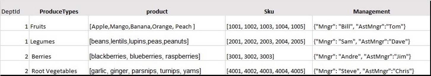
Table 1: Showing sample Data.
Let's create the Produce table as below.
hive>
DROP TABLE IF EXISTS Produce;
Create Table Produce(DeptId int, ProduceType string,
Product      array<string>,
Sku          array<int>,
Management   map<string, string>
)
row format delimited
fields terminated by '|'
collection items terminated by ','
map keys terminated by ':'
lines terminated by '\n' stored as textfile;
In the following step we load the table with Produce.txt text file.
LOAD DATA LOCAL INPATH 'C:\temp\Produce.txt' OVERWRITE INTO TABLE Produce;
EXPLODE
The EXPLODE() UDTF takes in an ARRAY or a MAP as an input and outputs the elements of these inputs as separate rows. As an example of using EXPLODE() in the SELECT expression list, the function is applied to the product column which has an ARRAY data type as shown below.
hive>
SELECT EXPLODE(Product) AS produce
FROM Produce;
Results:
OK
Apple
Mango
Banana
Orange
Peach
beans
…………..
Time taken: 33.255 seconds, Fetched: 18 row(s)
The results shows how each single row in the Produce column is transformed into multiple output rows.
In the next example below, the function is applied to the Management column which has a MAP data type:
hive>
SELECT EXPLODE (Management) AS (Mgr, AstMgr)
FROM Produce;
Results:
OK
Mngr    Bill
AstMngr Tom
Mngr    Sam
AstMngr Dave
Mngr    Andre
AstMngr Jim
Mngr    Steve
AstMngr Chris
Time taken: 14.172 seconds, Fetched: 8 row(s)
POSEXPLODE
POSEXPLODE() is similar to EXPLODE but instead of just returning the elements of the ARRAY it returns the element as well as its position in the original array. As an example of using POSEXPLODE() in the SELECT expression list as shown below:
Hive>
SELECT POSEXPLODE (Product) AS (Position, Product)
FROM Produce;
Results:
OK
0       Apple
1       Mango
2       Banana
3       Orange
4       Peach
.........
Time taken: 15.232 seconds, Fetched: 18 row(s)
As we can see, elements of the produce as well as their position in the original ARRAY are returned in the results.
The use of these functions has some limitations as outlined below;
- No other expressions are allowed in SELECT. In other words
SELECT DeptId, Explode(Product) AS Product...
is not supported.
- UDTF's can't be nested.
SELECT Explode(Explode(Product)) AS Product...
This is not supported.
- GROUP BY / CLUSTER BY / DISTRIBUTE BY / SORT BY are not supported.
There alternative ways around the UDTF limitations by using what is refered to as like LateralViews in Hive (LateralViews).
When you implement a lateral view, it first applies the UDTF to each row of a base table to generate the multiple rows from the individual rows. It then joins resulting output rows to the input rows to form a virtual table having the supplied table alias.
A LATERAL VIEW with explode() can be used to convert Product into separate rows in conjunction to with the other columns in the table as shown in the query:
hive>
SELECT DeptId, ProduceType, Prod
FROM Produce LATERAL VIEW explode(Produce) ProdTable AS prod;
Results:
OK
1       Fruits                Apple
1       Fruits                Mango
1       Fruits                Banana
..      …………                  …………
2       RootVegetables          parsnips
2       RootVegetables          turnips
2       RootVegetables          yams
Time taken: 16.505 seconds, Fetched: 18 row(s)
We can count the number of produce each department is selling as below:
hive>
SELECT DeptId, Count(Prod)
FROM Produce LATERAL VIEW explode(Produce) ProdTable AS prod
Group By DeptId;
Results:
OK
1       10
2       8
Time taken: 30.6 seconds, Fetched: 2 row(s)
HiveQL implements a lot of other functions including comprehensive window and analytics functions very similar to other matured SQL Dialect. A complete list of these function can be found here.
Hive Streaming
In a previous article we looked at Hadoop streaming as an alternative way to transform data using a language other than Java. Hadoop streaming API opens an I/O pipe to these external processes. Even though Hive streaming works the same way as Hadoop streaming, Hive Streaming does not leverage that API. Hive implements its streaming rather through several clauses, namely MAP(), REDUCE(), and TRANSFORM() .
In the Hadoop ecosystem, MAP and REDUCE could be mistaken for explicitly forcing Mapping or Reducing phases in the underlying MapReduce Jobs during streaming, which is not necessarily the case. In other words the REDUCE() clause in the query does not force a reduce phase to occur neither does the word MAP clause force a new map phase.
The TRANSFORM() clause has the same functionalities as the MAP and REDUCE, so you could use only that to avoid confusion as we will do in the following examples. Primarily, these option offers users the ability to plug in their own custom scripts in the data stream by using features natively supported in Hive and combine them with some SQL operations.
In lexical analytics, tokenization is the process of breaking a stream of text up into words, phrases, symbols, or other meaningful elements called tokens. In the following example we will use a python script tokenize.py to stream the tokenized content of a table SourceTble loaded with some text file. Here is the script
import sys
import re
for lineFeed in sys.stdin:
   for word in re.sub( r"['_,!.]",'',linefeed ).split():
     print "%s\t%d" % (word, 1)
The simple script strips off the text of unwanted characters using python regex to remove some characters and then splits the rows into a key value pair with the words as a key and a value of 1 as the value.
In the following step we create a new table called stopwords and load it with stopwords (common words like “I, me, my, myself, the, we...”) that we will like to filter out of most lexical analysis.
hive>
DROP TABLE IF EXISTS StopWords;
hive>
CREATE TABLE StopWords(StopWord STRING);
LOAD DATA LOCAL INPATH 'C:\temp\StopWords.txt' OVERWRITE INTO TABLE StopWords;
Let's check a few of the stop words.
hive>
SELECT StopWord from StopWords LIMIT 20;
Results:
OK
i
me
my
myself
we
our
ours
….
Next, we create a table called SourceTble and load it with some text. In this example the text we use is a text file containing the 1805 speech of Thomas Jefferson.
hive>
DROP TABLE IF EXISTS SourceTble;
hive>
CREATE TABLE SourceTble(Lines STRING);
LOAD DATA LOCAL INPATH 'C:\Temp\1805-Jefferson.txt' OVERWRITE INTO TABLE SourceTble;
In the next step we use the TRANFORM streaming task to stream rows from the SourceTble applying the tokenize.py script to generate key value pairs from each row, which are then returned as the columns in the SELECT statement. The results from the SELECT subquery are aggregated as a new table called WordCount.
hive>
DROP TABLE IF EXISTS WordCount1;
hive>
CREATE TABLE WordCount1
AS select r.key as Word, Sum(r.value) as Cnt
FROM (
      SELECT TRANSFORM (lines)
      USING 'c:\python27\python.exe c:\hdp\hadoop-2.4.0.2.1.3.0-1981\tokenize.py'
      AS (key, value)
FROM SourceTble
) r
group by r.key order by (Cnt DESC);
Next, we select the Top 10 most frequent words excluding stop words.
hive>
SELECT wc.* FROM WordCount1 wc
left outer join Stopwords sw
on lower(wc.word) = lower(sw.Stopword)
WHERE sw.Stopword is Null
LIMIT 10;
Results;
OK
public                      14.0
may                         10.0
citizens                    10.0
fellow                      8.0
us                          7.0
among                       7.0
shall                       7.0
state                       6.0
limits                      5.0
Constitution                5.0
Time taken: 32.821 seconds, Fetched: 10 row(s)
The following example shows how multiple scripts can be applied in a query, still delegating the mapping and reducing to Hive. Here, the script Aggregate.py is used to aggregate the key/value pair from the initial stream from the tokenizer script.
hive>
CREATE TABLE WordCount2(word STRING, cnt INT)
ROW FORMAT DELIMITED FIELDS TERMINATED BY '\t';
hive> FROM (
FROM SourceTble
SELECT TRANSFORM (lines)
USING 'c:\python27\python.exe c:\hdp\hadoop-2.4.0.2.1.3.0-1981\tokenize.py'
AS word, cnt
CLUSTER BY word
) r
INSERT OVERWRITE TABLE WordCount2
  SELECT TRANSFORM (r.word, r.cnt)
  USING 'c:\python27\python.exe c:\hdp\hadoop-2.4.0.2.1.3.0-1981\aggregate.py'
  AS word, cnt
  order by(Cnt DESC);
It should be noted that streaming is less efficient than coding the equivalent as a User Defined Function or as mapReduce jobs with Java. For users who want to write code in a language other than Java, Hive streaming is an option. In that sense it is very useful for fast prototyping since you are able to leverage existing code in your language of choice. It is useful for data transformation in Hive ETL patterns and useful for creating some structure from unstructured data.
Conclusion
We've looked at patterns geared towards storing and analyzing Big Data or huge data files in their original formats on Hadoop clusters with SQL. Objectives which otherwise would have previously required Java MapReduce programing or some other new language. We also looked at patterns that permits in-depth SQL analytics on both cool and hot Big Data through Hive Managed Tables and External Tables.
The discussions also exposed some Big Data solutions that can capitalize on SQL for various ETL patterns in the cloud or on-premise data repositories with options to extend data transformation using your favorite programing languages in that process. This included techniques that can help scale workload and improve performance in the process.
All-in-all we learned that today, there are various ways to leverage SQL for ETL and to perform batch or interactive analytical queries on structured and semi-structured Big Data for various applications.